import numpy as np
from scipy import optimize
import matplotlib.pyplot as plt
from scipy.special import expit as sigmoid
from scipy import stats
from scipy.integrate import simpsonSur-Candes phase transition in logistic regression
Consider a logistic regression estimate \[ \hat\beta = \operatorname{argmin}_{b\in \mathbb R^p} \sum_{i=1}^n \log(1+\exp(-y_i x_i^T b)) \] where \(y_i\in\{-1,1\}\) are binary responses and \(x_i\in \mathbb R^p\) are feature vectors of dimension \(p\). If a binary logistic model holds, of the form \[x_i\sim N(0_p,I_p), \qquad P(y_i=1|x_i)=\frac{1}{1+\exp(-y_ix_i^T\beta^*)}\] for some ground truth \(\beta^*\in\mathbb R^p\) with \(\|\beta^*\|=\gamma\), Candès and Sur (2020) predicts the above optimization problem admits a solution if \[ \kappa < h(\gamma) = \min_{t\in \mathbb R} \mathbb E\Big[\max(0,t y_ix_i^T\beta^* + Z)^2\Big] \] where \(n,p\to+\infty\) simultaneously with limiting ratio \(\kappa=\lim(p/n)\) and \(Z\sim N(0,1)\) is independent of everything else; while if \[ \kappa > h(\gamma) \] then no minimizer exists. The expectation on the right-hand side, as well as its gradient with respect to \(t\mathbb R\), can be computed by numerical integration.
Solving the minimization using numerical integration
grid_integration_size = 60
gamma = 0.01 * (1.1 ** np.array(range(100))).reshape((-1, 1, 1, 1))
Z = np.linspace(-6,6, num=grid_integration_size).reshape((1, -1, 1, 1))
X = np.linspace(-6,6, num=grid_integration_size + 1).reshape((1, 1, -1, 1))
Y = np.array([1,-1]).reshape((1, 1, 1, 2))
conditional_pmf_Y = sigmoid(X*Y*gamma)


def E(x, keepdims=False):
    assert len(x.shape) == 4
    x = x * stats.norm.pdf(Z) * conditional_pmf_Y * stats.norm.pdf(X)
    x = np.sum(x, axis=3)
    x = simpson(x, x=X.squeeze(), axis=2)
    x = simpson(x, x=Z.squeeze(), axis=1)
    if keepdims:
        return x[..., np.newaxis, np.newaxis, np.newaxis]
    return x
Once we are able to integrate with respect to the joint distribution of \((Z,X,Y)\), we simply perform a gradient descent to find the minimum over \(t\). The gradient of \(t\mapsto \mathbb E\big[\max(0,t y_ix_i^T\beta^* + Z)^2\big]\) is given by \[ 2 \mathbb E[ y_ix_i^T\beta^* \max(0,t y_ix_i^T\beta^* + Z) ]. \] A simple gradient descent finds the scalar \(t\) achieving the minimum in the definition of \(h(\gamma)\).
# initialization
t = 10 * np.ones_like(gamma)
# gradient descent
for _ in range(500):
    t += - 2 * E(Y * X * np.clip(t * Y * X - Z, a_min=0, a_max=None), keepdims=True)

kappa = E(np.clip(t * Y * X - Z, a_min=0, a_max=None)**2)
plt.plot(kappa.squeeze(), gamma.squeeze(), label=r"curve $\kappa=h(\gamma)$")
plt.xlabel(r"$\kappa$")
plt.ylabel(r"$\gamma$")
plt.legend()
plt.ylim(0, 15)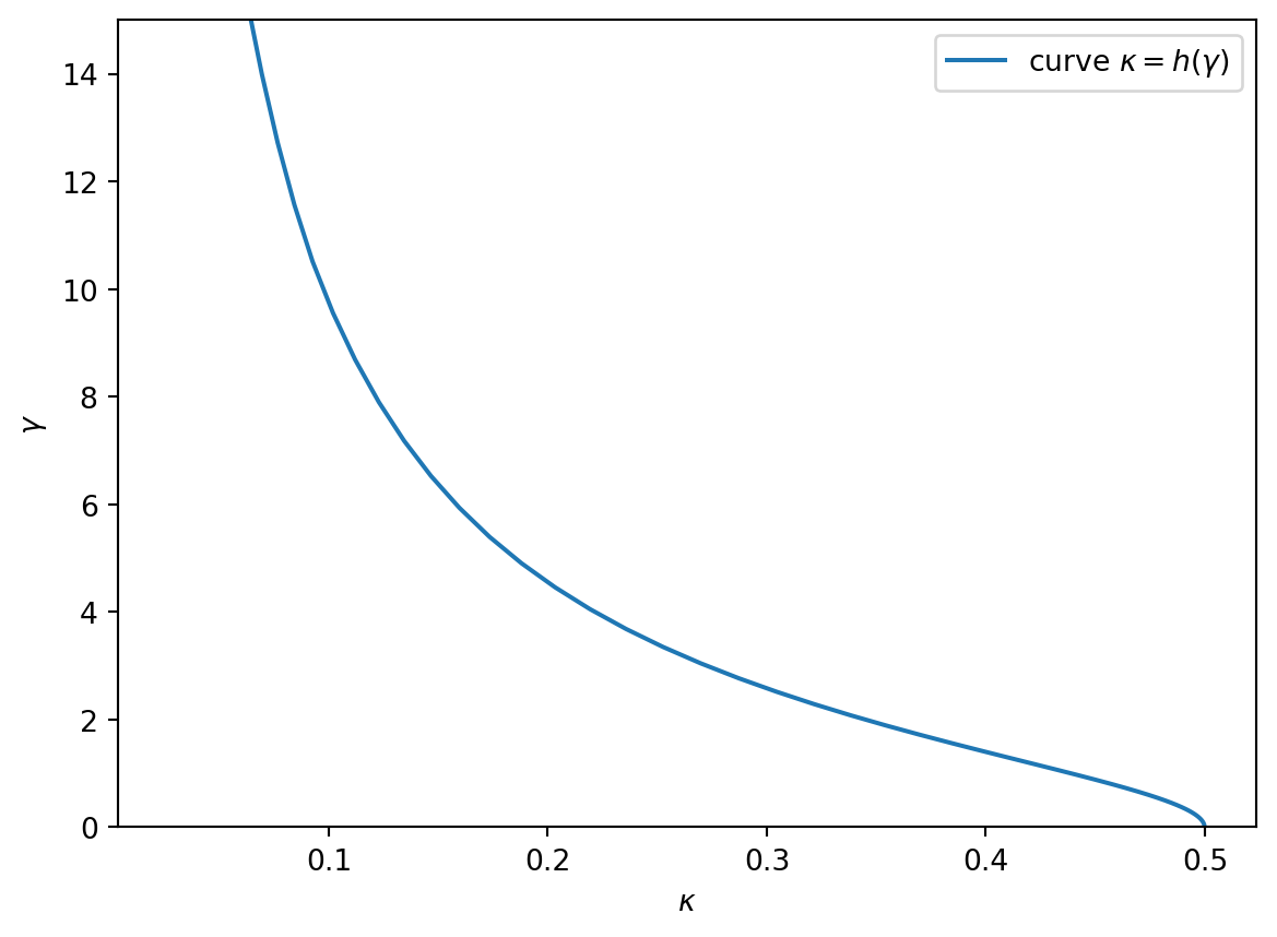
Simulation experiment
We now verify this phase transition empirically by verifying whether \[ \hat\beta = \operatorname{argmin}_{b\in \mathbb R^p} \sum_{i=1}^n \log(1+\exp(-y_i x_i^T b)) \] has a solution. The code below runs an iterative algorithm to solve the above optimization problem. Either the algorithm converges, or the the algorithm reaches the maximal number of iterations and returns a direction \(\hat b\) that perfectly separates the data, in the sense that \(\min_{i\in[n]} y_i \hat y_i \ge 0\) where \(\hat y_i = x_i\hat b\) for each observation \(i\in[n]\).
from sklearn.linear_model import LogisticRegression

def mle_exists(n, p, gamma, seed=2024):
    regr = LogisticRegression(penalty=None, fit_intercept=False)
    beta = gamma * np.ones(p)/np.sqrt(p)
    rng = np.random.default_rng(seed)
    X = rng.standard_normal(size=(n, p))
    y = - (-1) ** rng.binomial(1, sigmoid(X.dot(beta)))
    regr.fit(X, y)
    y_hat = X @ regr.coef_.reshape((p, ))
    return {'p': p, 'n': n, 'p':p, 'gamma': gamma, 'seed': seed, 'kappa': p/n,
            'MLE exists': not min(y * y_hat) >= 0.0}

mle_exists(1000, 200, 1.3)
{'p': 200,
'n': 1000,
'gamma': 1.3,
'seed': 2024,
'kappa': 0.2,
'MLE exists': True}We now experiment with \(n=1000\), dimension \(p\) ranging from 1 to \(n/2+50\), and \(\gamma\) parameters equispaced from 0 to 12. For each \((n,p,\gamma)\), the dataset is generated 10 times.
n = 1000
parameters = [{'n': 1000, 'p': p, 'gamma': g, 'seed': seed}
              for p in range(1, n//2 + 50, 5)
              for g in np.linspace(0, 12, num=100)
              for seed in range(10)]
from joblib import Parallel, delayed
f"Will now launch {len(parameters)} parallel tasks"'Will now launch 110000 parallel tasks'# Heavy parallel computation
data = Parallel(n_jobs=18, verbose=2)(delayed(mle_exists)(**d) for d in parameters)Visualizing the phase transition: theory versus empirical probabilities
Code
import pandas as pd
import matplotlib.pyplot as plt
import seaborn as sns
import matplotlib as mpl
mpl.rcParams['figure.dpi'] = 150

fig, (ax1, ax2) = plt.subplots(1, 2, gridspec_kw={'width_ratios': [1.2, 1]})
fig.set_size_inches(15, 5.5)

piv = pd.pivot_table(pd.DataFrame(data),
                     values='MLE exists',
                     index='gamma',
                     columns='kappa')
piv.unstack().reset_index().plot(x='kappa', y='gamma', c=0, kind='scatter', ax=ax1)
ax1.plot(kappa.squeeze(), gamma.squeeze(), color='red', label='theory', linewidth=3.0)
plt.xlabel('kappa = dimension / sample size')
plt.ylabel(r'gamma = $\sqrt{Var[x_i^T \beta^*]}$')
ax1.legend()

ax2.plot(kappa.squeeze(), gamma.squeeze(), color='red')
ax2.fill_between(kappa.squeeze(), gamma.squeeze(), color="yellowgreen")
maxy = ax2.get_ylim()[1]
ax2.fill_between(kappa.squeeze(), gamma.squeeze(), maxy, color="lightcoral")
ax2.fill_between(np.linspace(0.5, 0.6), np.zeros(50), maxy, color="lightcoral")


ax2.text(0.1, 2.0 ,"logistic MLE exists")
ax2.text(0.25, 5.0 ,"logistic MLE does not exist")

for ax in [ax1, ax2]:
    ax.set_ylabel(r'gamma = $\sqrt{Var[x_i^T \beta^*]}$')
    ax.set_xlabel('kappa = dimension / sample size')
    ax.set_xlim(0.02, 0.55)
    ax.set_ylim(0, 12)
    ax.margins(x=0, y=0)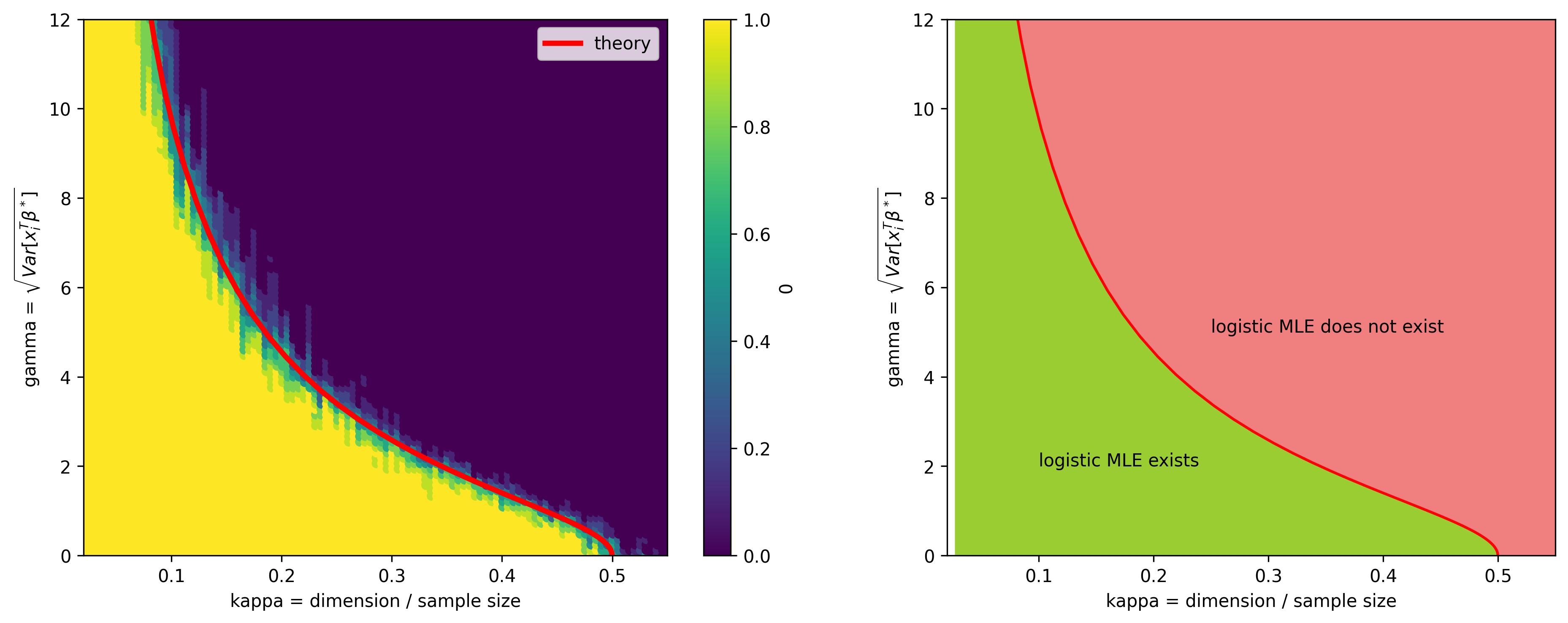
References
Candès, Emmanuel J, and Pragya Sur. 2020. “The Phase Transition for the Existence of the Maximum Likelihood Estimate in High-Dimensional Logistic Regression.” Ann. Statist. 48 (1): 27–42.