import numpy as np
from numpy.linalg import norm
import matplotlib.pyplot as plt

n = 10000                   # sample size
p = 15000                   # dimension
s = 1000                    # sparsity
T = 100                     # number of iterations
eta = (1+np.sqrt(p/n))**-2 # learning rate
L = 1/eta                  # smoothness of the loss
lam = 0.01                 # tuning parameter
sigma = 1.5                # noise level

# true regression vector
beta = 15 * np.hstack([np.ones(s), np.zeros(p-s)]) / np.sqrt(n)

# data generation process
rng = np.random.default_rng(2025)
X = rng.standard_normal(size=(n, p)) # feature matrix
y = X @ beta + sigma * rng.standard_normal(size=(n, )) # signal + noiseEstimating the generalization performance of an iterative algorithm along its trajectory
In a linear model \(y_i = x_i^T\beta + \epsilon_i\) with true regression vector \(\beta\in\mathbb R^p\), noise \(\epsilon_i\sim N(0,\sigma^2)\) and feature matrix \(X\in \mathbb R^{n\times p}\) with rows \((x_i)_{i\in [n]}\), we are interested in estimationg the generalization error of an iterative algorithm of the form \[\begin{equation} \hat b^t = g_t \Big( \hat b^{t-1},~\hat b^{t-2},~ \frac{X^T(y - X\hat b^{t-1})}{n},~ \frac{X^T(y-X\hat b^{t-2}}{n}) \Big) \end{equation}\] for some function \(g_t\) of the two previous iterates and their gradients (here, with respect to the square loss). The iterate and gradient at iteration \(t-2\) are included to allow for accelerated methods that require momentum.
The following example illustrates the estimator proposed in (Bellec and Tan 2025).
Proximal Gradient Descent
In the simple example below, we focus on the proximal gradient descent (Parikh, Boyd, et al. 2014) iterates \[\begin{equation} \hat b^t = g \Big( \hat b^{t-1} + \frac{\eta X^T(y-X\hat b^{t-1}}{n}) \Big) \end{equation}\] where \(\eta>0\) is a learning rate parameter, and the nonlinear function \(g\) is the proximal operator of the L1 norm with parameter \(\eta \lambda\), namely, the soft-thresholding \[\begin{equation} g(u) = \text{soft}(u; v), \text{ where } v=\lambda\eta \text{ and } \text{soft}(u; v) = \text{sign}(u)(|u| - v)_+. \end{equation}\]
def soft(x, t):
    return np.sign(x)*np.clip(np.abs(x)-t, 0, None)

plt.plot(np.linspace(-3,3), soft(np.linspace(-3, 3), 2))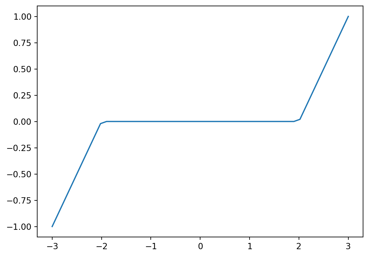
Hutchinson’s trace approximation
We will use the following trick to efficiently estimate the trace of a large matrix: if \(R = (r_{ik})_{i\in[n],k=[m]}\) has iid symmetric \(\pm 1/\sqrt m\), then for \(Q\in \mathbb R^{n\times n}\) the Hutchinson approximation \(\text{trace}(Q)\approx\text{trace}(R^TQR)/m\) holds with \(m\) of constant order provided \(\|Q\|_F \lll \text{trace}(Q)\).
m = 10
r = rng.choice([-1.0, 1.0], size=(n, m)) / np.sqrt(m)
For instance, let us verify this approximation with a random matrix:
G = rng.normal(size=(n, n))
temporary_matrix = G.T @ np.diag(np.linspace(1, 10, num=n)) @ G
np.trace(temporary_matrix), np.trace(r.T @ temporary_matrix @ r)(550122897.8034426, 550825944.5616682)Estimating the generalization error along the algorithm trajectory
We are now ready to compute the iterates of the proximal gradient algorithm, as well as the estimate of its generalization error from (Bellec and Tan 2025).
# initialization of arrays
F = np.zeros((n, T))                   # residuals
H = np.zeros((p, T), dtype=np.float16) # error vectors
bt = np.zeros_like(beta)               # iterate
F[:, 0] = y - X @ bt
H[:, 0] = bt - beta
A = np.zeros((T, T))                   # memory matrix
XTr = X.T @ r                          # r has iid Rademacher entries

for t in range(1, T):
    print(t, end="..")
    bt = soft(bt + eta * X.T @ (y-X@bt) /n, lam * eta)
    Dt = np.zeros(p, dtype=bool)
    Dt[np.nonzero(bt)[0]] = 1
    Dt = Dt.reshape((p, 1))
    if t >= 1:
        Rt = Dt * XTr if t == 1 else np.hstack([Dt * (Rt - (eta/n)*X.T @ ( X @ Rt)), Dt * XTr])
        A[t, :t] = np.trace((eta * XTr.T @ Rt / n).reshape((m, t, m)),
                            axis1=0, axis2=2)

    F[:, t] = y - X @ bt
    H[:, t] = bt - beta

M = np.linalg.solve(np.eye(T)-A/n, F.T).T
generalization_error = H.T @ H + np.ones((T, T))*sigma**2
generalization_error_estimate = M.T @ M/n1..2..3..4..5..6..7..8..9..10..11..12..13..14..15..16..17..18..19..20..21..22..23..24..25..26..27..28..29..30..31..32..33..34..35..36..37..38..39..40..41..42..43..44..45..46..47..48..49..50..51..52..53..54..55..56..57..58..59..60..61..62..63..64..65..66..67..68..69..70..71..72..73..74..75..76..77..78..79..80..81..82..83..84..85..86..87..88..89..90..91..92..93..94..95..96..97..98..99..import pandas as pd
df = pd.DataFrame(np.column_stack([
np.diag(generalization_error_estimate),
np.diag(generalization_error),
]))
df.columns = ('generalization error', 'estimate of the generalization error')
df.plot()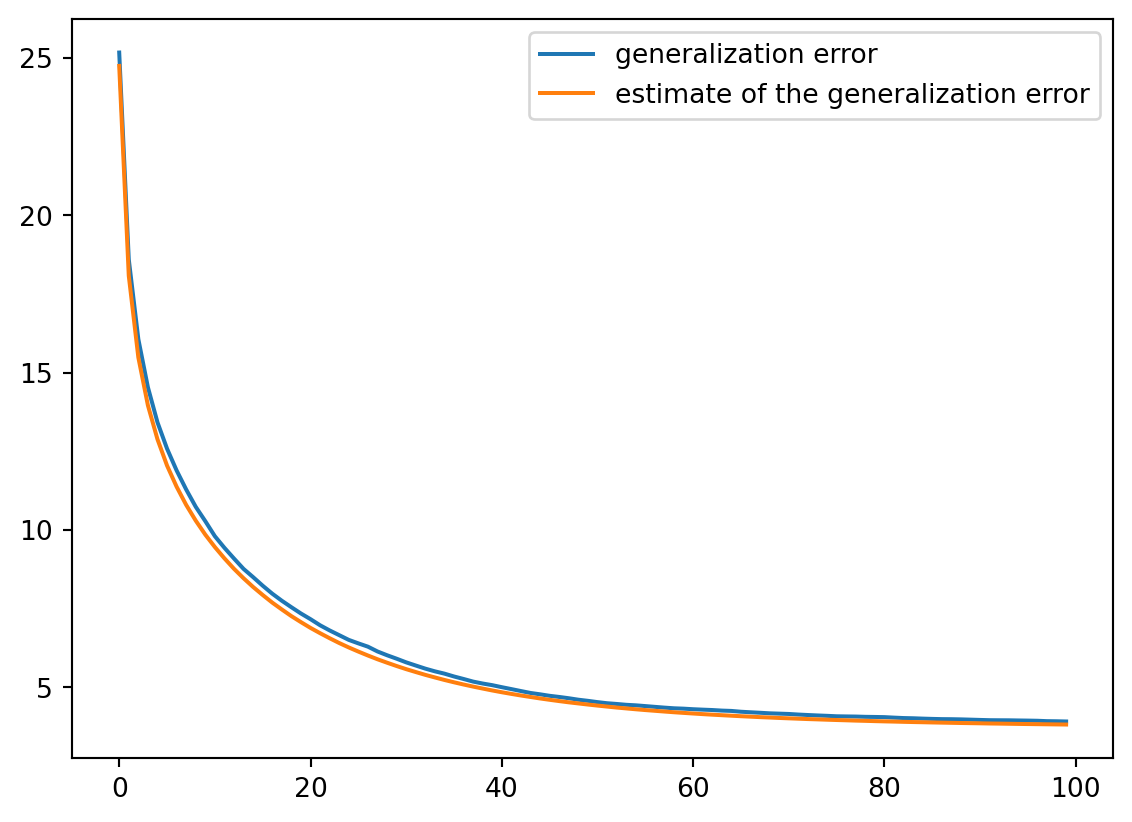
df.round(2)| generalization error | estimate of the generalization error | |
|---|---|---|
| 0 | 25.18 | 24.75 |
| 1 | 18.60 | 18.08 |
| 2 | 16.06 | 15.48 |
| 3 | 14.53 | 13.96 |
| 4 | 13.42 | 12.88 |
| ... | ... | ... |
| 95 | 3.94 | 3.83 |
| 96 | 3.94 | 3.83 |
| 97 | 3.92 | 3.82 |
| 98 | 3.92 | 3.82 |
| 99 | 3.91 | 3.82 |
100 rows × 2 columns
References
Bellec, Pierre C, and Kai Tan. 2025. “Uncertainty Quantification for Iterative Algorithms in Linear Models with Application to Early Stopping.” Ann. Statist., in Press. https://arxiv.org/pdf/2404.17856.
Parikh, Neal, Stephen Boyd, et al. 2014. “Proximal Algorithms.” Foundations and Trends in Optimization 1 (3): 127–239.